What is J-Curve In Economics?
Understand the J-Curve in economics, how it explains trade balance changes, and its impact on currency and economic policies.

Introduction to the J-Curve in Economics
The J-Curve is a useful concept in economics that explains how a country's trade balance reacts over time to changes in currency value or trade policies. If you’ve ever wondered why a currency depreciation might initially worsen a trade deficit before improving it, the J-Curve provides the answer.
In this article, we’ll explore what the J-Curve is, why it matters, and how it affects economic decisions. Understanding this concept can help you grasp the dynamics behind trade balances and currency fluctuations.
What is the J-Curve Effect?
The J-Curve describes the pattern of a country’s trade balance following a depreciation or devaluation of its currency. Initially, the trade deficit tends to worsen before it improves, creating a shape similar to the letter 'J' when graphed over time.
- Initial Worsening:
Right after depreciation, import prices rise, making imports more expensive in local currency terms.
- Delayed Improvement:
Over time, exports become cheaper for foreign buyers, increasing export volumes.
- Net Effect:
Eventually, the trade balance improves as export growth outweighs import costs.
This time lag happens because contracts and consumer habits don’t adjust immediately to price changes.
How Does the J-Curve Work?
When a currency loses value, the cost of imported goods rises instantly. However, the quantity of imports and exports takes time to respond. Here’s how the process unfolds:
- Short-Term Impact:
Import bills increase, worsening the trade deficit.
- Medium-Term Adjustment:
Exporters become more competitive internationally, boosting sales.
- Long-Term Result:
The trade balance improves as export growth exceeds import costs.
This delayed response is why the trade balance initially dips before rising, forming the J-shaped curve.
Examples of the J-Curve in Real Economies
Several countries have experienced the J-Curve effect after currency depreciation or trade policy changes. Here are some examples:
- United Kingdom (1992):
After the pound was devalued, the UK’s trade deficit initially worsened but improved after exports picked up.
- Turkey (2018):
The lira’s sharp depreciation led to a short-term trade deficit spike before export growth helped narrow it.
- Japan (1990s):
Yen depreciation showed a delayed positive effect on trade balance consistent with the J-Curve theory.
These examples highlight how the J-Curve plays out in different economic contexts.
Why is the J-Curve Important for Economic Policy?
Understanding the J-Curve helps policymakers anticipate the short-term pain and long-term gain from currency adjustments or trade reforms.
- Timing Expectations:
Policymakers can prepare for initial trade deficits after devaluation.
- Policy Design:
Helps in designing complementary policies to support exporters during the adjustment period.
- Market Confidence:
Clear communication about the J-Curve effect can stabilize markets during volatile periods.
Ignoring the J-Curve can lead to misjudging the impact of currency moves and trade policies.
Factors Influencing the J-Curve Effect
The strength and duration of the J-Curve depend on several factors:
- Price Elasticity:
How sensitive importers and exporters are to price changes affects the speed of adjustment.
- Contract Lengths:
Long-term contracts delay the response of trade volumes to price changes.
- Economic Structure:
Countries with diverse export bases may see quicker improvements.
- Global Demand:
Strong foreign demand can accelerate export growth after depreciation.
These factors determine how pronounced the J-Curve will be in any economy.
Limitations of the J-Curve Concept
While the J-Curve is a helpful model, it has limitations you should keep in mind:
- Not Universal:
Some countries may not experience a clear J-Curve due to unique economic conditions.
- Short-Term Volatility:
Other factors like inflation or capital flows can mask the J-Curve effect.
- Assumes Rational Behavior:
The model assumes that trade volumes adjust logically, which may not always happen.
It’s important to view the J-Curve as one tool among many for understanding trade dynamics.
Conclusion
The J-Curve in economics explains why a country’s trade balance often worsens before it improves following currency depreciation. This pattern results from the delayed response of import and export volumes to price changes.
By understanding the J-Curve, you can better grasp the complexities of trade balances and currency effects. This knowledge is valuable for investors, policymakers, and anyone interested in international economics.
FAQs about the J-Curve in Economics
What causes the initial worsening in the J-Curve?
The initial worsening happens because import prices rise immediately after currency depreciation, increasing the cost of imports before export volumes can adjust.
How long does the J-Curve effect usually last?
The duration varies but typically lasts several months to a few years, depending on contract lengths and price elasticity.
Can the J-Curve effect be seen in all countries?
No, the effect depends on economic structure, trade policies, and market responsiveness; some countries may not show a clear J-Curve.
Why is price elasticity important for the J-Curve?
Price elasticity determines how quickly importers and exporters change their buying and selling behavior in response to price changes, influencing the J-Curve’s shape.
How do policymakers use the J-Curve concept?
Policymakers use it to anticipate trade balance changes after currency moves and to design supportive measures for exporters during adjustment periods.